The book Solid State Physics by the authors Ashcroft and Mermin is, together with Kittel, one of the classic textbooks in the field of solid state physics. Recently, I decided I wanted to brush up my knowledge on this subject and picked up the book.
The first chapter in the book concerns the simplistic Drude model, a purely classical model of electrical conduction. In the Drude model, conduction electrons are assumed to bounce arround randomly inside a static lattice of ions. Based on a few simple assumptions, the model is able to provide qualitative explanations for Ohm's law, the Hall effect, the plasma frequency and plasmons. Following the chapter, including the mathematical derivations, felt relatively straightforward. After reading the chapter, I had the feeling I understood the Drude model.
However, to have an honest grapple with the subject material and get the most out of these types of books, one has to solve the problems at the end of chapters. As is common with old textbooks, the very first problem in this book smacks you in the face with its high difficulty (I guess in the 70's, students were expected to master mathematics at a much higher level). It was at this point I knew that, in fact, I did not understand the Drude model.
Maybe I'm not as good at math as I'd like to believe, but I spent multiple hours on this problem. At many points I was ready to give up and tried to find solutions online. None of the solutions I found gave me that satisfactory "oooh I get it now" feeling. So gradually, through trial and error, googling, ChatGPT discussions, and looking at various online solutions, I finally feel like "I get it". Since I haven't found a comprehensive discussion of this problem elsewhere online, I thought I would write it up here.
Let's dive in. The problem states:
1. Poisson Distribution:
In the Drude model the probability of an electron suffering a collision in any infinitesimal interval dt is just dt/τ.
(a) Show that an electron picked at random at a given moment had no collision during the preceding t seconds with probability e-t/τ. Show that it will have no collision during the next t seconds with the same probability.
For one electron, we can draw a timeline from time 0 to \(t\), which we divide into \(N\) slices of width \(dt\). Because the time at which we picked out the electron is random, we can arbitrarily choose the time to be \(t\), so that our timeline starts at time 0.
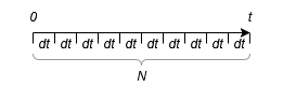
The chance our electron has a collision in a time interval \(dt\) is \(dt/\tau\). This means that the chance our electron does not have a collision in \(dt\) is \(1 - dt/\tau\). Because each time interval is independent, the chance that our electron has no collision in the entire \([0,t]\) interval is:
We know that \(t = N dt\), which we can use to substitute for \(dt\):
Since time is a continuum, we want to take the limit of this expression as \(N \to \infty\) (or as \(dt \to 0\)). Notice that this is the exact same expression as \(e^x\) (see Wikipedia), with \(x=-t/\tau\). Hence:
This proves the statement and solves the problem.
To prove that the probability of no collision is the same for the next \(t\) seconds is trivial. We can pick out the electron at time 0 instead and follow the same math to come up with exactly the same result.
(b) Show that the probability that the time interval between two successive collisions of an electron falls in the range between \(t\) and \(t+dt\) is \((dt/\tau)e^{-t/\tau}\).
The wording of this question is very tricky. Essentially we are interested in the time gaps between successive collisions. Imagine if we look at each collision of an electron, one by one, and center each at time 0. Then we look for the next collision and find it at time, say, \(t_i\). The question is asking what the probability is that \(t \leq t_i \leq t + dt\).
With this reframing of the question, the solution becomes easy. Essentially the probability that \(t \leq t_i \leq t + dt\) is the probability that no collisions happen between 0 and \(t\) (\(=e^{-t/\tau}\)) and then a collision occurs between \(t\) and \(t+dt\) (=\(dt/\tau\)). Therefore, the probability is:
This is what needed to be demonstrated.
(c) Show as a consequence of (a) that at any moment the mean time back to the last collision (or up to the next collision) averaged over all electrons is \(\tau\).
Let's introduce a random variable \(X\) that represents the time back to the last collision for an electron (or the time to the next collision). In this problem, we are trying to find the expected value of \(X\). To get the expected value of a continuous random variable \(X\), we need the probability density function, which we will now derive.
From (a) we know that the probability of no collision happening in the previous \(t\) is \(e^{-t/\tau}\). The "probability that no collision happens in the previous \(t\)", is the same as saying "the probability of a collision happening at a time back greater than \(t\)". Expressed in mathematical notation:
By the rules of probability, we know that:
This is essentially just saying that the probabilities for all possible values of \(X\) need to add up to 1. This means that:
Put in words, the chance of the time to the next collision being smaller than \(t\) is equal to this expression.
Notice that this expression looks very much like a cumulative distribution function for the continuous random variable \(X\). We can obtain the probability density function \(f(t)\) by taking the derivative of the CDF with respect to \(t\):
The mean of \(X\), \(E[X]\) can now be calculated by evaluating the following integral:
We can evaluate this using integration by parts:
As a side note, the probability distribution we have derived here is the exponential distribution, which describes the distance between events in a Poisson process. The electron collisions in the Drude model are a Poisson process: the chance of a collision happening is constant in an infinitesimal interval of time. The title of the problem is quite misleading, since we are not dealing with the Poisson distribution at all. The Poisson distribution describes how many events occur in a fixed amount of time. The exponential distribution is basically the mirror image: how much time occurs between events.
(d) Show as a consequence of (b) that the mean time between successive collisions of an electron is \(\tau\).
Let \(Y\) be the random variable that represents the time between successive collisions of an electron. If time gaps would be discrete, the expected time gap between collisions would be expressed as
where \(P(t_i)\) is the probability that the gap is equal to \(t_i\).
Since time gaps are continuous, this becomes an integral:
We know from (b) that
so:
This is the same integral as in (c), with the same answer: \(\tau\).
Notice the subtlety in the question and framing: in (a) and (c), we are concerned with calculating the probabilities and expected time until the previous (or the next) collision of all the electrons. In parts (b) and (d), we are concerned with the probabilities and expected gaps between successive collisions of a single electron. The real "trick" is that, at each arbitrary moment in time, the probability distribution for the next collision of an electron is identical. Therefore, if we choose an arbitrary electron at any moment in time, the expected time to the next collision is \(\tau\). But a collision is also an arbitrary moment in time, so the average time until the next collision, and thus the inter-collision spacing, is also \(\tau\).
(e) Part (c) implies that at any moment the time \(T\) between the last and next collision averaged over all electrons is \(2\tau\). Explain why this is not inconsistent with the result in (d). (A thorough explanation should include a derivation of the probability distribution for \(T\).) A failure to appreciate this sublety led Drude to a conductivity only half of (1.6). He did not make the same mistake in the thermal conductivity, whence the factor of two in his calculation of the Lorenz number (see page 23).
This is by far the most tricky part of the problem and requires careful reading and analysis.
Essentially, the question points to an apparent paradox. If we take a random electron, the expected time since the last collision is \(\tau\) and the expected time until the next collision is also \(\tau\). Therefore, we would expect that, on average over all electrons, the time between the last and the next collision should be \(2\tau\). However, we showed in (d) that the average inter-collision spacing of an electron is \(\tau\).
Let's define the random variable \(T\), which describes the time between the last and the next collision. The time to the last collision is described by the random variable \(X\) (see part (c)), and so is the time to the next collision. Therefore \(T = X_1 + X_2\).
When adding random variables, we can calculate the probability density function of the resulting random variable using the convolution of the original PDFs. In our case, this takes the following form:
A critical detail here is the apparent change of the upper integration bound from \(\infty\) to \(t\) and the lower bound from \(-\infty\) to \(0\). The reason the upper integrand bound changes is best explained by imagining the convolution graphically. In the convolution, one of the functions is flipped across the y axis and then "slid accross" the other function. At each position, the functions are multiplied together and the result is integrated. The result is a function that represents the integral of the multiplied functions as a function of slide position.
The reason our integral starts at 0 and goes up to \(t\), is that our PDF is only nonzero on the interval \([0, \infty]\); on the interval \([-\infty, 0]\), the PDF is 0. So, in actuality, our PDF is a piecewise function. Taking this fact into account yields these integration bounds.
In any case, we now have an expression for the PDF of random variable \(T\). To calculate the expected value (mean), we again have to evaluate an integral:
This can be evaluated by using integration by parts twice:
Of course this is the complicated way to do it; we could have also just observed that \(E[T] = E[X] + E[X] = 2\tau\), but it's nice to get confirmation.
So this is saying that when we choose a random moment in time, the times from the previous collision to the next collision for all electrons will follow the probability distribution \(f_T(t)\) which we derived, with an expected mean value of \(2\tau\). This distribution is known as the Erlang distribution.
How does this not contradict the result in (d)? The key elements to the question is "at any moment in time" and "averaged over all electrons". In (d), we look at all collisions and observe the time to the next collision. In this part of the question, we take a snapshot at a specific moment in time and observe the length of the inter-collision time intervals we intersect with. The reason the average interval we observe in this case is greater than \(\tau\), is simply because we have a higher chance of intersecting with longer intervals. Consider two intervals in two different electrons: one of length 1 and the other of length 10. If we pick a random moment in time, we will have a 10 times higher chance of landing in the second interval. This gives us an intuitive explanation for why the factor \(t\) appears in the PDF: it represents the bias of landing in longer time intervals. The exponential factor represents the probability of longer intervals appearing over time in our population of electrons, which counteracts the bias to longer intervals since longer intervals are more rare.
To really drive home the point, we can demonstrate these things with a simple Monte Carlo simulation in Python. We generate a long array of random floating point numbers between 0 and 1. This represents a discretized timeline for a single electron, each element in the array representing a segment \(dt\).
import numpy as np

N = 100000000
timeline = np.random.rand(N)
Let's say that all values smaller than 0.01 are considered collisions.
This allows us to generate a boolean array with collision events represented with True:
collision_chance = 0.01  # = 1/tau
collisions = timeline < collision_chance
We are now interested in the inter-collision spacing.
First we find the indices where collisions == True:
collision_indices = np.where(collisions)[0]
We can calculate the inter-collision intervals as follows:
intervals = collision_indices[1:] - collision_indices[:-1]
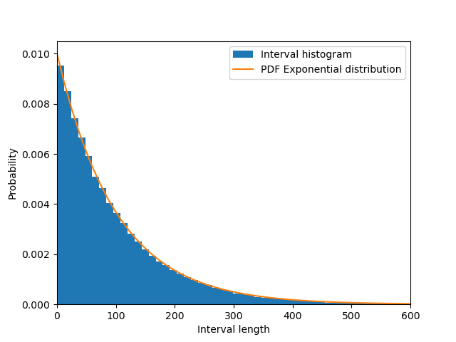
Plotting a histogram of the intervals, we get our expected exponential distribution:
import matplotlib.pyplot as plt

x_lower = 0
x_upper = 600

fig, ax = plt.subplots(1)
ax.hist(intervals, 100, density=True, label="Interval histogram")

# the expected PDF in the limit
x = np.linspace(0, x_upper)
y = chance * np.exp(-x * chance)
ax.plot(x, y, label="PDF Exponential distribution")
ax.set_xlim(x_lower, x_upper)

ax.set_xlabel("Interval length")
ax.set_ylabel("Probability")

ax.legend()

Also calculating the mean using np.mean retrieves us the expected 100 (=1/0.01).
However, now let's sample time randomly. We can do this by generating a large array of random integers that reference an element in the original array:
time_samples = np.random.randint(0, N, size=1000000)
To extract the "interval size" each time sample corresponds to, we create an array that contains the interval size at each element:
interval_data = np.empty(N, dtype=int)
for i in range(len(intervals)):
    interval_data[collision_indices[i]:collision_indices[i+1]] = intervals[i]
end_gap = collision_indices[0] + (len(interval_data) - collision_indices[-1])
interval_data[:collision_indices[0]] = end_gap
interval_data[collision_indices[-1]:] = end_gap
We include the first collision in the interval and exclude the second collision. To deal with the first and last intervals, we use periodic boundary conditions and assume it is the same interval that "wraps around".
Then we obtain the interval size corresponding to the time sample as follows:
sampled_intervals = interval_data[time_samples]
We can again make a histogram plot and find it corresponds to the expected Erlang distribution:
import matplotlib.pyplot as plt

x_lower = 0
x_upper = 800

fig, ax = plt.subplots(1)
ax.hist(sampled_intervals, 100, density=True, label="Interval histogram")

# the expected PDF in the limit
x = np.linspace(0, x_upper)
y = chance ** 2 * x * np.exp(-x * chance)
ax.plot(x, y, label="PDF Erlang distribution")
ax.set_xlim(x_lower, x_upper)

ax.set_xlabel("Interval length")
ax.set_ylabel("Probability")

ax.legend()
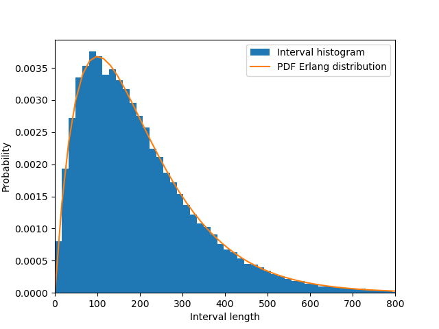
Calculating the mean of sampled_intervals yields the expected value around 200 (2\(\tau\)).
Note that here we look at the timeline of a single electron and sample it at different times, while the question deals with an average over multiple electrons at one point in time. However, the calculation is identical: all electrons have an equivalent timeline, so sampling the same timeline at different points is the same as sampling multiple timelines at one point.
The previous discussion corroborates our findings in (d) and (e).
For completeness, we can also calculate the times to the previous (and next) collision at our random time samples to corroborate the findings in (c).
To do so, we replace interval_data with the index of the start of the interval:
interval_data = np.empty(N, dtype=int)
for i in range(len(intervals)):
    interval_data[collision_indices[i]:collision_indices[i+1]] = collision_indices[i]
interval_data[:collision_indices[0]] = collision_indices[-1] - len(interval_data)
interval_data[collision_indices[-1]:] = collision_indices[-1]
We can now calculate the time to the start of the interval for each time sample as follows:
time_to_previous = time_samples - interval_data[time_samples]
If we draw a histogram of this data as before, we again retrieve our expected exponential distribution:
The mean again comes out to close to 100, as expected. An identical analysis can be performed for the times to the end of the interval.
So finally, let's tie it back to the mistake that Drude made. The question and chapter suggests Drude found a conductivity \(\sigma\) half of the expression in 1.6, which is expressed as:
The conductivity scales linearly with \(\tau\), so this implies Drude used half of the value of \(\tau\) somehow. How exactly he made this mistake is difficult to say without reading his papers, given that \(\tau\) actually refers to the time since the last collision averaged over all electrons.
Comments
Currently the comment submission form is not active. You can add a comment via pull request.There are no comments on this article yet.